Build a crop segmentation machine learning model with Planet data and Amazon SageMaker geospatial capabilities

This guest post is co-written by Lydia Lihui Zhang, Business Development Specialist, and Mansi Shah, Software Engineer/Data Scientist, at Planet Labs. The analysis that inspired this post was originally written by Jennifer Reiber Kyle.

Amazon SageMaker geospatial capabilities combined with Planet’s satellite data can be used for crop segmentation, and there are numerous applications and potential benefits of this analysis to the fields of agriculture and sustainability. In late 2023, Planet announced a partnership with AWS to make its geospatial data available through Amazon SageMaker.

Crop segmentation is the process of splitting up a satellite image into regions of pixels, or segments, that have similar crop characteristics. In this post, we illustrate how to use a segmentation machine learning (ML) model to identify crop and non-crop regions in an image.

Identifying crop regions is a core step towards gaining agricultural insights, and the combination of rich geospatial data and ML can lead to insights that drive decisions and actions. For example:

• Making data-driven farming decisions – By gaining better spatial understanding of the crops, farmers and other agricultural stakeholders can optimize the use of resources, from water to fertilizer to other chemicals across the season. This sets the foundation for reducing waste, improving sustainable farming practices wherever possible, and increasing productivity while minimizing environmental impact.
• Identifying climate-related stresses and trends – As climate change continues to affect global temperature and rainfall patterns, crop segmentation can be used to identify areas that are vulnerable to climate-related stress for climate adaptation strategies. For example, satellite imagery archives can be used to track changes in a crop growing region over time. These could be the physical changes in size and distribution of croplands. They could also be the changes in soil moisture, soil temperature, and biomass, derived from the different spectral index of satellite data, for deeper crop health analysis.
• Assessing and mitigating damage – Finally, crop segmentation can be used to quickly and accurately identify areas of crop damage in the event of a natural disaster, which can help prioritize relief efforts. For example, after a flood, high-cadence satellite images can be used to identify areas where crops have been submerged or destroyed, allowing relief organizations to assist affected farmers more quickly.

In this analysis, we use a K-nearest neighbors (KNN) model to conduct crop segmentation, and we compare these results with ground truth imagery on an agricultural region. Our results reveal that the classification from the KNN model is more accurately representative of the state of the current crop field in 2017 than the ground truth classification data from 2015. These results are a testament to the power of Planet’s high-cadence geospatial imagery. Agricultural fields change often, sometimes multiple times a season, and having high-frequency satellite imagery available to observe and analyze this land can provide immense value to our understanding of agricultural land and quickly-changing environments.

Planet and AWS’s partnership on geospatial ML

SageMaker geospatial capabilities empower data scientists and ML engineers to build, train, and deploy models using geospatial data. SageMaker geospatial capabilities allow you to efficiently transform or enrich large-scale geospatial datasets, accelerate model building with pre-trained ML models, and explore model predictions and geospatial data on an interactive map using 3D-accelerated graphics and built-in visualization tools. With SageMaker geospatial capabilities, you can process large datasets of satellite imagery and other geospatial data to create accurate ML models for various applications, including crop segmentation, which we discuss in this post.

Planet Labs PBC is a leading Earth-imaging company that uses its large fleet of satellites to capture imagery of the Earth’s surface on a daily basis. Planet’s data is therefore a valuable resource for geospatial ML. Its high-resolution satellite imagery can be used to identify various crop characteristics and their health over time, anywhere on Earth.

The partnership between Planet and SageMaker enables customers to easily access and analyze Planet’s high-frequency satellite data using AWS’s powerful ML tools. Data scientists can bring their own data or conveniently find and subscribe to Planet’s data without switching environments.

Crop segmentation in an Amazon SageMaker Studio notebook with a geospatial image

In this example geospatial ML workflow, we look at how to bring Planet’s data along with the ground truth data source into SageMaker, and how to train, infer, and deploy a crop segmentation model with a KNN classifier. Finally, we assess the accuracy of our results and compare this to our ground truth classification.

The KNN classifier used was trained in an Amazon SageMaker Studio notebook with a geospatial image, and provides a flexible and extensible notebook kernel for working with geospatial data.

The Amazon SageMaker Studio notebook with geospatial image comes pre-installed with commonly used geospatial libraries such as GDAL, Fiona, GeoPandas, Shapely, and Rasterio, which allow the visualization and processing of geospatial data directly within a Python notebook environment. Common ML libraries such as OpenCV or scikit-learn are also used to perform crop segmentation using KNN classification, and these are also installed in the geospatial kernel.

Data selection

The agricultural field we zoom into is located at the usually sunny Sacramento County in California.

Why Sacramento? The area and time selection for this type of problem is primarily defined by the availability of ground truth data, and such data in crop type and boundary data, is not easy to come by. The 2015 Sacramento County Land Use DWR Survey dataset is a publicly available dataset covering Sacramento County in that year and provides hand-adjusted boundaries.

The primary satellite imagery we use is the Planet’s 4-band PSScene Product, which contains the Blue, Green, Red, and Near-IR bands and is radiometrically corrected to at-sensor radiance. The coefficients for correcting to at-sensor reflectance are provided in the scene metadata, which further improves the consistency between images taken at different times.

Planet’s Dove satellites that produced this imagery were launched February 14, 2017 (news release), therefore they didn’t image Sacramento County back in 2015. However, they have been taking daily imagery of the area since the launch. In this example, we settle for the imperfect 2-year gap between the ground truth data and satellite imagery. However, Landsat 8 lower-resolution imagery could have been used as a bridge between 2015 and 2017.

Access Planet data

To help users get accurate and actionable data faster, Planet has also developed the Planet Software Development Kit (SDK) for Python. This is a powerful tool for data scientists and developers who want to work with satellite imagery and other geospatial data. With this SDK, you can search and access Planet’s vast collection of high-resolution satellite imagery, as well as data from other sources like OpenStreetMap. The SDK provides a Python client to Planet’s APIs, as well as a no-code command line interface (CLI) solution, making it easy to incorporate satellite imagery and geospatial data into Python workflows. This example uses the Python client to identify and download imagery needed for the analysis.

You can install the Planet Python client in the SageMaker Studio notebook with geospatial image using a simple command:

%pip install planet

You can use the client to query relevant satellite imagery and retrieve a list of available results based on the area of interest, time range, and other search criteria. In the following example, we start by asking how many PlanetScope scenes (Planet’s daily imagery) cover the same area of interest (AOI) that we define earlier through the ground data in Sacramento, given a certain time range between June 1 and October 1, 2017; as well as a certain desired maximum cloud coverage range of 10%:

# create a request using the SDK from the search specifications of the data

item_type = ['PSScene']

geom_filter_train = data_filter.geometry_filter(aoi_train)
date_range_filter = data_filter.date_range_filter("acquired", gt=datetime(month=6, day=1, year=2017), lt=datetime(month=10, day=1, year=2017))
cloud_cover_filter = data_filter.range_filter('cloud_cover', lt=0.10)

combined_filter_test = data_filter.and_filter([geom_filter_test, date_range_filter, cloud_cover_filter])
    
# Run a quick search for our TRAIN data
async with Session() as sess:
    cl = sess.client('data')
    results = cl.search(name='temp_search_train',search_filter=combined_filter_train, item_types=item_type)
    train_result_list = [i async for i in results]

print("Number of train scene results: ", len(train_result_list))

The returned results show the number of matching scenes overlapping with our area of interest. It also contains each scene’s metadata, its image ID, and a preview image reference.

After a particular scene has been selected, with specification on the scene ID, item type, and product bundles (reference documentation), you can use the following code to download the image and its metadata:

train_scene_id = '20170601_180425_0f35'
item_type = 'PSScene'
bundle_type = 'analytic_sr_udm2'

# define the order request
products = [order_request.product([train_scene_id], bundle_type, item_type)]
request = order_request.build_request('train_dataset', products=products)

# download the training data
async with Session() as sess:
    cl = sess.client('orders')
    # use "reporting" to manage polling for order status
    with reporting.StateBar(state='creating') as bar:
        # perform the order with the prior created order request
        order = await cl.create_order(request)
        bar.update(state='created', order_id=train_order['id'])

        # wait via polling until the order is processed
        await cl.wait(train_order['id'], callback=bar.update_state)

    #  download the actual asset
    await cl.download_order(order_id=order['id'], directory=download_directory, progress_bar=True, overwrite=True)

This code downloads the corresponding satellite image to the Amazon Elastic File System (Amazon EFS) volume for SageMaker Studio.

Model training

After the data has been downloaded with the Planet Python client, the segmentation model can be trained. In this example, a combination of KNN classification and image segmentation techniques is used to identify crop area and create georeferenced geojson features.

The Planet data is loaded and preprocessed using the built-in geospatial libraries and tools in SageMaker to prepare it for training the KNN classifier. The ground truth data for training is the Sacramento County Land Use DWR Survey dataset from 2015, and the Planet data from 2017 is used for testing the model.

Convert ground truth features to contours

To train the KNN classifier, the class of each pixel as either crop or non-crop needs to be identified. The class is determined by whether the pixel is associated with a crop feature in the ground truth data or not. To make this determination, the ground truth data is first converted into OpenCV contours, which are then used to separate crop from non-crop pixels. The pixel values and their classification are then used to train the KNN classifier.

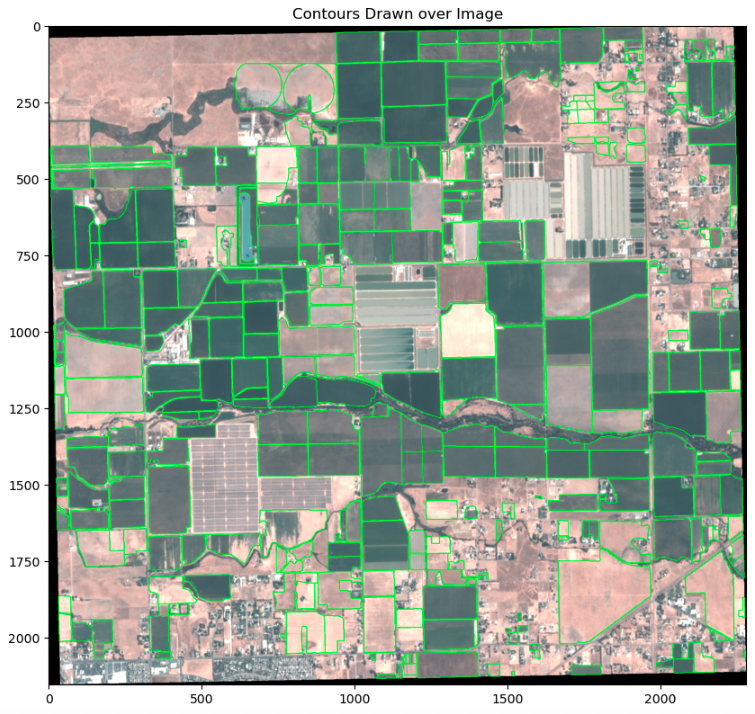
To convert the ground truth features to contours, the features must first be projected to the coordinate reference system of the image. Then, the features are transformed into image space, and finally converted into contours. To ensure the accuracy of the contours, they are visualized overlaid on the input image, as shown in the following example.

To train the KNN classifier, crop and non-crop pixels are separated using the crop feature contours as a mask.

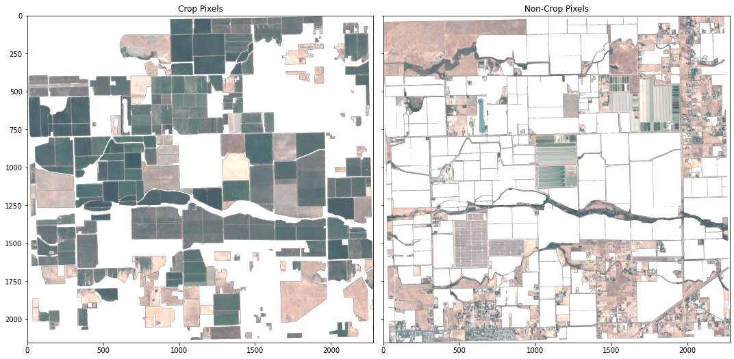
The input of KNN classifier consists of two datasets: X, a 2d array that provides the features to be classified on; and y, a 1d array that provides the classes (example). Here, a single classified band is created from the non-crop and crop datasets, where the band’s values indicate the pixel class. The band and the underlying image pixel band values are then converted to the X and y inputs for the classifier fit function.

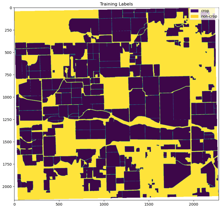
Train the classifier on crop and non-crop pixels

The KNN classification is performed with the scikit-learn KNeighborsClassifier. The number of neighbors, a parameter greatly affecting the estimator’s performance, is tuned using cross-validation in KNN cross-validation. The classifier is then trained using the prepared datasets and the tuned number of neighbor parameters. See the following code:

def fit_classifier(pl_filename, ground_truth_filename, metadata_filename, n_neighbors):
    weights = 'uniform'
    clf = neighbors.KNeighborsClassifier(n_neighbors, weights=weights)
    train_class_band = create_contour_classified_band(pl_filename, ground_truth_filename)
    X = to_X(load_refl_bands(pl_filename, metadata_filename))
    y = to_y(train_class_band)
    clf.fit(X, y)
    return clf

clf = fit_classifier(train_scene_filename,
                     train_ground_truth_filename,
                     train_metadata_filename,
                     n_neighbors)

To assess the classifier’s performance on its input data, the pixel class is predicted using the pixel band values. The classifier’s performance is mainly based on the accuracy of the training data and the clear separation of the pixel classes based on the input data (pixel band values). The classifier’s parameters, such as the number of neighbors and the distance weighting function, can be adjusted to compensate for any inaccuracies in the latter. See the following code:

def predict(pl_filename, metadata_filename, clf):
    bands = load_refl_bands(pl_filename, metadata_filename)
    X = to_X(bands)
    y = clf.predict(X)
    return classified_band_from_y(bands[0].mask, y)

train_predicted_class_band = predict(train_scene_filename, train_metadata_filename, clf)

Evaluate model predictions

The trained KNN classifier is utilized to predict crop regions in the test data. This test data consists of regions that were not exposed to the model during training. In other words, the model has no knowledge of the area prior to its analysis and therefore this data can be used to objectively evaluate the model’s performance. We start by visually inspecting several regions, beginning with a region that is comparatively noisier.

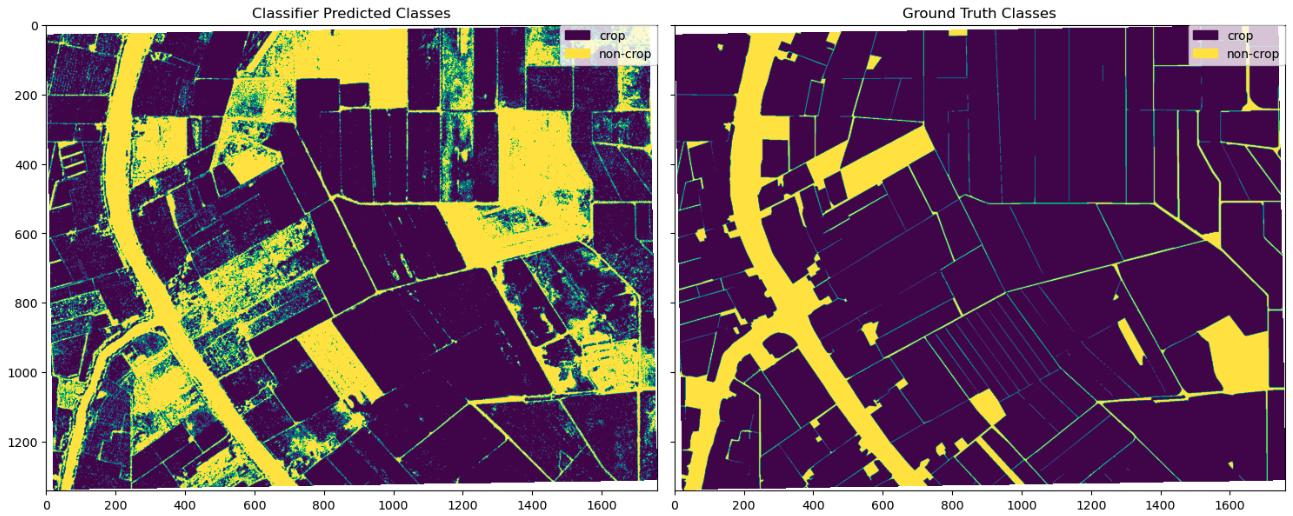
The visual inspection reveals that the predicted classes are mostly consistent with the ground truth classes. There are a few regions of deviation, which we inspect further.

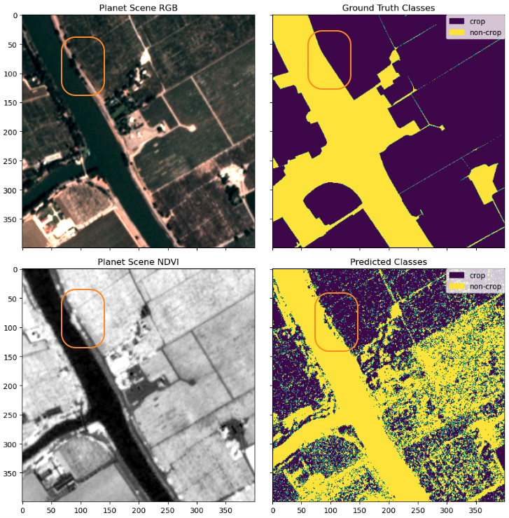
Upon further investigation, we discovered that some of the noise in this region was due to the ground truth data lacking the detail that is present in the classified image (top right compared to top left and bottom left). A particularly interesting finding is that the classifier identifies trees along the river as non-crop, whereas the ground truth data mistakenly identifies them as crop. This difference between these two segmentations may be due to the trees shading the region over the crops.

Following this, we inspect another region that was classified differently between the two methods. These highlighted regions were previously marked as non-crop regions in the ground truth data in 2015 (top right) but changed and shown clearly as cropland in 2017 through the Planetscope Scenes (top left and bottom left). They were also classified largely as cropland through the classifier (bottom right).

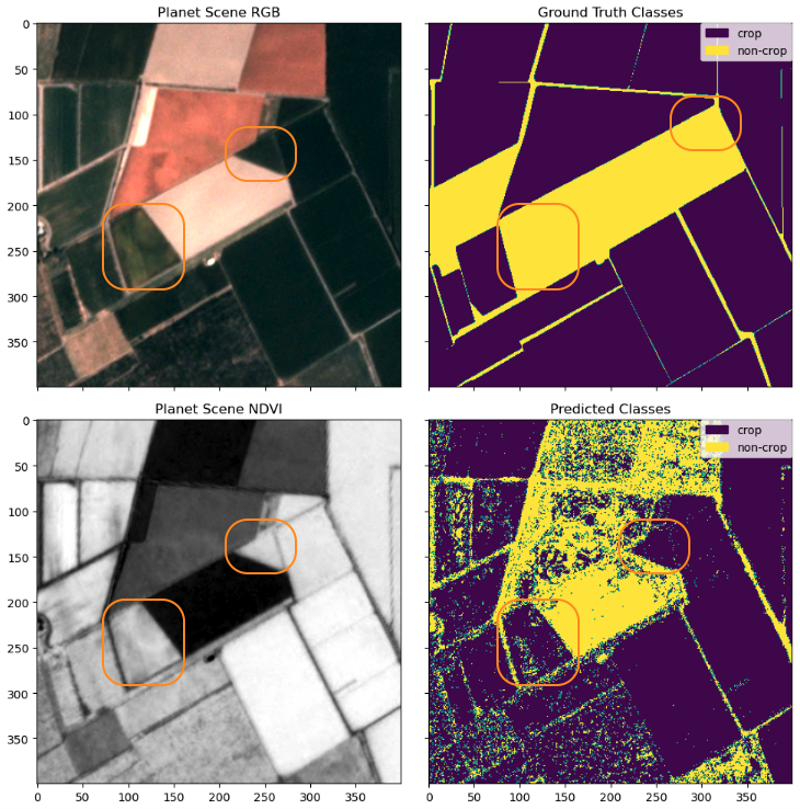
Again, we see the KNN classifier presents a more granular result than the ground truth class, and it also successfully captures the change happening in the cropland. This example also speaks to the value of daily refreshed satellite data because the world often changes much faster than annual reports, and a combined method with ML like this can help us pick up the changes as they happen. Being able to monitor and discover such changes via satellite data, especially in the evolving agricultural fields, provides helpful insights for farmers to optimize their work and any agricultural stakeholder in the value chain to get a better pulse of the season.

Model evaluation

The visual comparison of the images of the predicted classes to the ground truth classes can be subjective and can’t be generalized for assessing the accuracy of the classification results. To obtain a quantitative assessment, we obtain classification metrics by using scikit-learn’s classification_report function:

# train dataset
print(classification_report(to_y(create_contour_classified_band(train_scene_filename,
                                          train_ground_truth_filename)),
                            to_y(train_predicted_class_band),
                            target_names=['crop', 'non-crop']))

              precision    recall  f1-score   support

        crop       0.89      0.86      0.87   2641818
    non-crop       0.83      0.86      0.84   2093907

    accuracy                           0.86   4735725
   macro avg       0.86      0.86      0.86   4735725
weighted avg       0.86      0.86      0.86   4735725



# test dataset
print(classification_report(to_y(create_contour_classified_band(test_scene_filename,
                                       test_ground_truth_filename)),
                            to_y(test_predicted_class_band),
                            target_names=['crop', 'non-crop']))

              precision    recall  f1-score   support

        crop       0.94      0.73      0.82   1959630
    non-crop       0.32      0.74      0.44    330938

    accuracy                           0.73   2290568
   macro avg       0.63      0.74      0.63   2290568
weighted avg       0.85      0.73      0.77   2290568

The pixel classification is used to create a segmentation mask of crop regions, making both precision and recall important metrics, and the F1 score a good overall measure for predicting accuracy. Our results give us metrics for both crop and non-crop regions in the train and test dataset. However, to keep things simple, let’s take a closer look at these metrics in the context of the crop regions in the test dataset.

Precision is a measure of how accurate our model’s positive predictions are. In this case, a precision of 0.94 for crop regions indicates that our model is very successful at correctly identifying areas that are indeed crop regions, where false positives (actual non-crop regions incorrectly identified as crop regions) are minimized. Recall, on the other hand, measures the completeness of positive predictions. In other words, recall measures the proportion of actual positives that were identified correctly. In our case, a recall value of 0.73 for crop regions means that 73% of all true crop region pixels are correctly identified, minimizing the number of false negatives.

Ideally, high values of both precision and recall are preferred, although this can be largely dependent on the application of the case study. For example, if we were examining these results for farmers looking to identify crop regions for agriculture, we would want to give preference to a higher recall than precision, in order to minimize the number of false negatives (areas identified as non-crop regions that are actually crop regions) in order to make the most use of the land. The F1-score serves as an overall accuracy metric combining both precision and recall, and measuring the balance between the two metrics. A high F1-score, such as ours for crop regions (0.82), indicates a good balance between both precision and recall and a high overall classification accuracy. Although the F1-score drops between the train and test datasets, this is expected because the classifier was trained on the train dataset. An overall weighted average F1 score of 0.77 is promising and adequate enough to try segmentation schemes on the classified data.

Create a segmentation mask from the classifier

The creation of a segmentation mask using the predictions from the KNN classifier on the test dataset involves cleaning up the predicted output to avoid small segments caused by image noise. To remove speckle noise, we use the OpenCV median blur filter. This filter preserves road delineations between crops better than the morphological open operation.

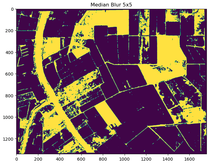
To apply binary segmentation to the denoised output, we first need to convert the classified raster data to vector features using the OpenCV findContours function.

Finally, the actual segmented crop regions can be computed using the segmented crop outlines.

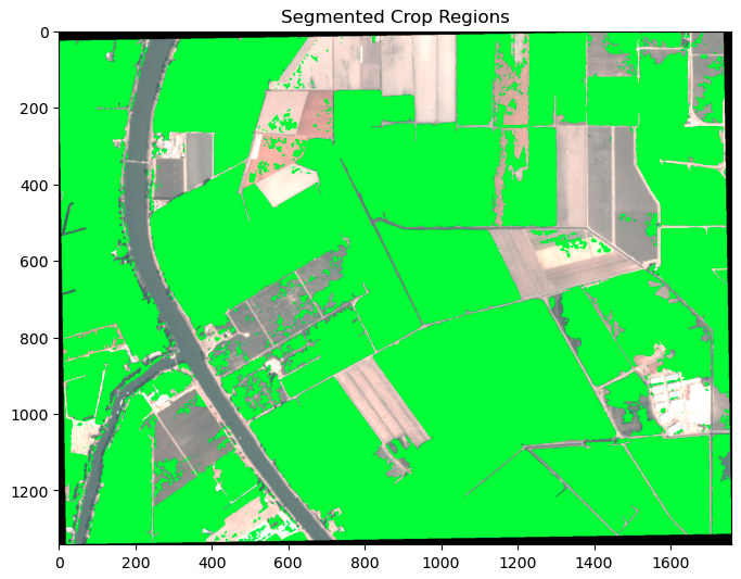
The segmented crop regions produced from the KNN classifier allow for precise identification of crop regions in the test dataset. These segmented regions can be used for various purposes, such as field boundary identification, crop monitoring, yield estimation, and resource allocation. The achieved F1 score of 0.77 is good and provides evidence that the KNN classifier is an effective tool for crop segmentation in remote sensing images. These results can be used to further improve and refine crop segmentation techniques, potentially leading to increased accuracy and efficiency in crop analysis.

Conclusion

This post demonstrated how you can use the combination of Planet’s high cadence, high-resolution satellite imagery and SageMaker geospatial capabilities to perform crop segmentation analysis, unlocking valuable insights that can improve agricultural efficiency, environmental sustainability, and food security. Accurately identifying crop regions enables further analysis on crop growth and productivity, monitoring of land use changes, and detection of potential food security risks.

Moreover, the combination of Planet data and SageMaker offers a wide range of use cases beyond crop segmentation. The insights can enable data-driven decisions on crop management, resource allocation, and policy planning in agriculture alone. With different data and ML models, the combined offering could also expand into other industries and use cases towards digital transformation, sustainability transformation, and security.

To start using SageMaker geospatial capabilities, see Get started with Amazon SageMaker geospatial capabilities.

To learn more about Planet’s imagery specifications and developer reference materials, visit Planet Developer’s Center. For documentation on Planet’s SDK for Python, see Planet SDK for Python. For more information about Planet, including its existing data products and upcoming product releases, visit https://www.planet.com/.

Planet Labs PBC Forward-Looking Statements

Except for the historical information contained herein, the matters set forth in this blog post are forward-looking statements within the meaning of the “safe harbor” provisions of the Private Securities Litigation Reform Act of 1995, including, but not limited to, Planet Labs PBC’s ability to capture market opportunity and realize any of the potential benefits from current or future product enhancements, new products, or strategic partnerships and customer collaborations. Forward-looking statements are based on Planet Labs PBC’s management’s beliefs, as well as assumptions made by, and information currently available to them. Because such statements are based on expectations as to future events and results and are not statements of fact, actual results may differ materially from those projected. Factors which may cause actual results to differ materially from current expectations include, but are not limited to the risk factors and other disclosures about Planet Labs PBC and its business included in Planet Labs PBC’s periodic reports, proxy statements, and other disclosure materials filed from time to time with the Securities and Exchange Commission (SEC) which are available online at www.sec.gov, and on Planet Labs PBC’s website at www.planet.com. All forward-looking statements reflect Planet Labs PBC’s beliefs and assumptions only as of the date such statements are made. Planet Labs PBC undertakes no obligation to update forward-looking statements to reflect future events or circumstances.

About the authors

Lydia Lihui Zhang is the Business Development Specialist at Planet Labs PBC, where she helps connect space for the betterment of earth across various sectors and a myriad of use cases. Previously, she was a data scientist at McKinsey ACRE, an agriculture-focused solution. She holds a Master of Science from MIT Technology Policy Program, focusing on space policy. Geospatial data and its broader impact on business and sustainability have been her career focus.

Mansi Shah is a software engineer, data scientist, and musician whose work explores the spaces where artistic rigor and technical curiosity collide. She believes data (like art!) imitates life, and is interested in the profoundly human stories behind the numbers and notes.

Xiong Zhou is a Senior Applied Scientist at AWS. He leads the science team for Amazon SageMaker geospatial capabilities. His current area of research includes computer vision and efficient model training. In his spare time, he enjoys running, playing basketball, and spending time with his family.

Janosch Woschitz is a Senior Solutions Architect at AWS, specializing in geospatial AI/ML. With over 15 years of experience, he supports customers globally in leveraging AI and ML for innovative solutions that capitalize on geospatial data. His expertise spans machine learning, data engineering, and scalable distributed systems, augmented by a strong background in software engineering and industry expertise in complex domains such as autonomous driving.

Shital Dhakal is a Sr. Program Manager with the SageMaker geospatial ML team based in the San Francisco Bay Area. He has a background in remote sensing and Geographic Information System (GIS). He is passionate about understanding customers pain points and building geospatial products to solve them. In his spare time, he enjoys hiking, traveling, and playing tennis.